Forecasting Recessions from a Broad, Lag-Aligned Signal Panel, and the Case for a Forward-Horizon Disruption-Impulse Signal
Michael Landis
StratMac
Strategic.Macroeconomics@gmail.com
Abstract
AI disclosure. This working paper was researched and drafted with substantial use of an automated AI research assistant (DeepSeek 2.5 Flash); full disclosure in the Declaration of Generative AI (§11) and the Compliance & Provenance Appendix (§13). The human author takes responsibility for its content.
We build a config-driven, five-stage recession-forecasting pipeline for the United States that integrates (i) a broad monthly panel of continuously-valued economic series sourced through FRED, (ii) frequency-domain and cross-correlation lead/lag discovery, (iii) lag-aligned transfer-function and probabilistic models with walk-forward validation, (iv) a data-driven anomaly scan that recovers disruption episodes without any catalog, and (v) — the methodological contribution — a shock-catalog → disruption-impulse → forward-horizon significance framework for discrete policy/regulatory/biological shocks that have no continuous FRED series.
Three findings stand out. First, the forward-horizon method resolves a genuine identification problem: a tariff/trade-policy impulse shows ≈0 coincident correlation with recession onset (none of the three in-sample tariff episodes landed on a recession start) yet a positive leading signature peaking at +0.55 at an 18-month horizon — consistent with an uncertainty → capex-deferral → slowdown transmission channel. We are deliberately precise about the strength of this evidence: it rests on only n=3 trade episodes (53 active months) that are themselves autocorrelated within episode, so at the effective sample size the observed r=+0.55 carries a moving-block bootstrap 95% CI of [−0.138, +0.841] and a circular-shift permutation p≈0.08. It is therefore reported as a directionally consistent but statistically inconclusive lead — a hypothesis the method generates and future tariff episodes must confirm, not an established result. Coincident cross-correlation would have pronounced trade-policy shocks "useless"; the forward-horizon test reveals them as the class of shock that leads. Second, the same method cleanly separates leads from coincidences among the other shock families: energy oils correlate at +0.63 at +13 months coincidentally but flip negative forward (−0.38 at 3 months) — i.e. inside the recession window, not a long lead; biological shocks drop from +0.74 to +0.39 once the COVID outlier's dominance is recognized; regulatory phase-outs are weak and slow (no usable impulse timing). Third, a comprehensive robustness examination (labour-market tightness/Beveridge signals, an extended ±72-month lag search, and the pooling of individually-weak signals) confirms the breadth of the search and identifies the few genuinely long-lead continuous series — housing (−36 months) and the term spread (beyond +24) — while showing labour-tightness and cost-of-money measures are confirmatory rather than independently leading at a long horizon (§3, §4).
We conclude that a forward-horizon disruption-impulse index is a viable, quantitatively-grounded recession signal for the classes of shock that transmit slowly (notably trade/tariff policy), and we specify its construction and integration into the lag-aligned model. Critically, we subject the implemented index to out-of-sample validation against realised recessions (§6.2): it fired into 2004 and 2020–21 with no recession, was silent into 2001 and 2007–08, and its current near-term elevation rests on a single ongoing tariff episode. It is therefore presented as a research instrument, not a production gauge; the path to production (breadth, a clean elevation→recession record, recalibrated regime hold) is specified. All results are reported with disclosed sample sizes; the small number of qualifying shocks (n=3 trade, n=53 active months) is an honest upper bound on the strength of evidence, and we state it plainly rather than over-claiming. Taken together, the findings point toward a possible — not demonstrated — structural ceiling: high-frequency, smoothly-varying series may be information-theoretically weak predictors of the asynchronous, discrete reversals that constitute recessions. We frame this explicitly as a hypothesis motivating future work (details in §10.1), not a proven diagnosis — since this paper's own proposal to gather more episodes and folds could narrow the bounds and keep the lag-correlation approach viable. The durable-looking successor is nonetheless to model and propagate the asynchronous triggers themselves — announcement/rule shocks through a sector cost-structure graph — rather than to keep lag-correlating the smooth series that merely reflect them; whether that path outweighs simply collecting more data is an open empirical question we intend to test.
Results at a glance (detail and uncertainty in §4–§8).
| Result | Value | Honest status |
|---|---|---|
| Trade/tariff impulse, coincident vs recession | r≈0.00 | No coincident signal — would read as "useless" |
| Trade/tariff impulse, forward-lead @ 18 mo | +0.55 (95% CI [−0.138, +0.841]; permutation p≈0.08) | Directionally consistent, statistically inconclusive (n=3 episodes) |
| Energy | coincident +0.63 @ +13 → forward −0.38 @ 3 | Coincident, not a long lead |
| Biological | +0.74 → +0.39 forward, flat all horizons | COVID-driven; not a repeatable lead |
| Regulatory | −0.17 coincident / −0.08 forward | Weak, no usable timing |
| Model B recession-probit AUC | Walk-forward ≈0.998 (0.9978), in-sample 0.9998 | Single fold, 18 OOS recession months — encouraging, not proven; also overconfident at top end (Brier 0.0301, top-bin 0.991 vs empirical 0.818) |
| Model A INDPRO transfer R² | 0.63 (adj ≈0.615); OOS RMSE 13.90 vs in-sample 9.48 | Within-sample fit; OOS penalty is the honest generalization gap |
| Implemented index out-of-sample | Fired into 2004 & 2020–21; silent into 2001 & 2007–08 | Not ready for prime time (§6.2) |
1. Introduction and motivation
The StratMac dashboard de-dollarizes and normalizes a large panel of macro series, then flags each by a trailing-window z-score / σ percentile. That layer answers "is this series currently far from its own normal?" It does not, by itself, say "does this state predict a recession, and how far ahead?" This paper documents a five-stage research pipeline built to answer exactly that second question, and — because the user explicitly rejected any "omniscient preference" in favor of a discipline of "look everywhere and measure significance" — the design is deliberately unsupervised, broad, and measurement-first: we scan the entire panel for leads, we test shocks we do not have data for by constructing them from an anchored catalog, and we report both what works and what fails.
The central tension the pipeline addresses:
Slow-transmitting economic shocks — trade-policy changes, regulatory phase-outs, certain biological outbreaks — have no clean, continuous monthly time series on any public repository. A forecast model built only on FRED series therefore cannot "see" them at all. Either we accept that blindness, or we make our own signal from historical evidence.
We chose the latter. The methodological risk is inventing magnitudes. We bound that by the rule stated in Section 4: shock magnitude is anchored to an observed economic footprint where one exists (a measured trade-flow loss, a price move, a headcount), and is explicitly flagged low-confidence where no clean proxy exists — never a fabricated share-of-GDP number.
2. Data
2.1 Source and access
All series are accessed through the FRED public CSV endpoint (fredgraph.csv?id=<SERIES>). FRED re-hosts data produced by BEA, BLS, Census, the Federal Reserve Board, the Chicago Fed, EIA, Freddie Mac, S&P/Case-Shiller, and the University of Michigan; we credit the producers, not the access channel. Series are cached locally so analyses are reproducible from a single fetch.
2.2 Panel construction
recession_sources.json defines 74+ candidate series with per-series normalization metadata: de-dollarization (ratio_of a GDP-type or CPI deflator), per-capita (POP), and transform (log, pct-change, real-oil pct-change). The panel spans approximately 1950–2026 at monthly frequency where available.
Series classes represented:
- Yield/term structure: T10Y3M, T10Y2Y, T10YFF, BAA10Y, AAA10Y, AAAFF, term premia.
- Financial conditions / credit: NFCI, NFCILEVERAGE, BAA, VIXCLS, HY OAS (current-state only), IG OAS (current-state only).
- Credit tightening ("cost of money"): DRTSCILM (SLOOS C&I loan tightening; quarterly, interpolated), PRIME, CPN3M.
- Monetary aggregates / balance sheet: M2SL/GDP, M1REAL, BOGMBASE, TOTRESNS.
- Labor: UNRATE, UNEMPLOY, CIVPART, UEMP15T26, UEMP27OV, UEMPMEAN, UEMPMED, IC4WSA, CCSA, MANEMP, AWHMAN, ICSA.
- Activity / production: INDPRO, TCU, RRSFS.
- Prices / inflation: CPIAUCSL, PPIENG, CPIENGSL, GASREGW, APU000074714.
- Energy: DCOILWTICO (real pct-change), DCOILBRENTEU, DHHNGSP.
- Equities: NASDAQCOM.
- Sentiment / expectations: UMCSENT.
- Trade flows (continuous proxies): IMPGS, BOPGSTB. (Marks no clean tariff-rate series exists; trade policy handled as event overlay — Section 4.)
2.3 Sample and data-admissibility criteria
Three criteria govern which series enter the model fitting set; they are analysis-design choices, and we report their consequences explicitly rather than eliding them:
- A business-cycle minimum of 120 months (10 years). Cross-correlation and walk-forward evaluation need enough full cycles to be meaningful; anything shorter is a poor estimate. This keeps the fitting set to the long monthly series (term spreads, credit, labor, money, activity, prices).
- Strictly monthly. A quarterly series in a monthly panel collapses the shared aligned matrix to its own (coarser) timestamps. Quarterly survey data (SLOOS credit tightening, DRTSCILM) is admitted by linear interpolation to monthly; genuinely quarterly output measures (GDP, real personal income) are held out of the panel and used only as continuous-activity reference.
- Beveridge / labour-market-tightness signals (from 2000.12, 307 months) are kept out of the full-history fitting matrix but are active components of the stage-6 index. The exclusion from the full-history model is a data-length decision (a 2001+ series would collapse the 1955+ aligned matrix to its own start), not a dismissal. Fetched and cross-correlated against the NBER recession dummy (Probe A), JOLTS job openings lead by ~9 months (r=−0.32), hires by ~10 months (r=−0.40), separations are ~coincident (r=+0.37). Crucially, a marginal-value test (invest_longlead.py) shows JOLTS job openings adds ~+0.04 to +0.09 held-out AUC on top of the strong baseline even within its own window — i.e. it is genuinely contributing, not merely corroborating. We therefore feed it as a current-state labour-tightness component of the stage-6 index (§6), acknowledging the 307-month window covers only two recessions, so its contribution is treated as supporting evidence rather than the load-bearing on its own.
HY/IG option-adjusted spreads are fetched but are short (≈36 months available from the public endpoint) and fall below the 120-month criterion; we keep them as current-state gauges and do not spectral-analyze them.
3. Methods
Stage 1 — Normalization & panel construction
Fetch each configured series from FRED and normalize to a common monthly panel: interpolate population/GDP/deflators to monthly; apply per-capita, de-dollarization (ratio to GDP or deflate by CPI/GDP-deflator), and log/pct-change/real transforms; interpolate quarterly survey series (DRTSCILM) to monthly. Emits a single monthly panel spanning ~1950–2026.
Stage 2 — Lead/lag discovery
For each panel series: detrend + Hann taper, FFT → power spectrum (dominant cycles), and cross-correlation against the NBER recession dummy scanning lags −24 to +24 months (initial pass), yielding a lead/lag rank and dominant business-cycle band. A deep extension to ±72 months (Probe B) verifies that no material longer-horizon lead was missed before the ±24 window (results in §4.2).
Stage-2 findings (computed by the private-repo pipeline; inputs public, code on request).
| signal | lead (mo, + = leads) | |r| | cycles |
|---|---|---|---|
| NFCI | +1 | 0.60 | 7.0, 3.5 y |
| NFCILEVERAGE | +2 | 0.57 | 4.3, 2.9 y |
| VIXCLS | 0 | 0.49 | 6.1, 3.3 y |
| UNRATE | −11 | 0.44 | 5.5, 6.5 y |
| T10Y3M | −21 | 0.37 | 5.6, 2.4 y |
| T10Y2Y | +18 | 0.35 | 5.6, 2.4 y |
| T10YFF | +9 | 0.48 | — |
| M2SL/GDP | +9 | 0.16 | 8.4, 5.2 y |
The coefficient signs follow Estrella–Mishkin: the term spread (T10Y3M) leads by ~21 months; the yield-curve-inversion → recession signature is recovered independently of prior art. Financial conditions (NFCI) are the strongest correlate but effectively coincident. Dominant business cycle ~5–7 years.
Stage 3 — Lag-aligned models, walk-forward validated
We fit two models on inputs lag-aligned by the stage-2-detected leads, using strictly past-known values:
- Model A — a distributed-lag (transfer function) on industrial-production growth (INDPRO Δ). Successively improved R² from 0.37 → 0.63 as credit/labor/energy classes were added; DRTSCILM (credit tightening) emerged as the single dominant coefficient (−12) once its quarterly cadence was interpolated.
- Model B — a ridge-regularized logistic recession probit, walk-forward-validated.
All model inputs are aligned strictly to past-known values: a signal that stage-2 identifies as leading recession by L months enters the forecast for month t at its value at t − L (never a future or coincident offset). This rules out look-ahead bias by construction. Model A's INDPRO transfer function reached R²=0.63; Model B's walk-forward evaluation is reported with its honest thinness in §4.3.
Stage 4 — Anomaly scan ("measure everywhere")
An unsupervised trailing-window z-score scan across every panel series, recovering disruption episodes from the data itself with no catalog: the 2008 credit-tightening spike (DRTSCILM), the 2020 M1/M2 surge, Fed balance-sheet expansion (TOTRESNS/BOGMBASE) in 2008, unemployment spikes at every post-war recession (1957, 1970, 1975, 1980, 1991, 2001, 2008, 2020), NFCI stress (2007–08), and the BAA credit-spread blowout (2008). This stage is the "measure everywhere" engine and independently triangulates the episodes we later test in Stage 5.
Stage 5 — Disruption-impulse significance (the forward-horizon method)
The problem. Trade-policy shifts (tariffs), regulatory phase-outs, and certain biological shocks have no monthly FRED series. We cannot model what we cannot fetch. Stage 5 therefore constructs our own monthly signal from a scored catalog.
Catalog + magnitude-anchoring rule. shock_catalog.json records each disruption episode with timing (start/peak/end), category (trade/regulatory/biological/energy), direction, mechanism, and a magnitude anchored to an observed economic footprint — a measured trade-flow loss, a price move, a headcount culled — or an explicit low-confidence flag where none exists. All current magnitudes are justified by an anchor; none are invented share-of-GDP numbers. From this, build_impulse convolves magnitudes with a symmetric rise-to-peak / decay profile into a continuous monthly disruption impulse.
Circularity guard. Shock dates and magnitudes were sourced independently of the outcome series: every entry is dated from external event records (legislation passage / tariff effective dates, standard oil-supply break dates, pandemic onset) and its magnitude from an observed footprint, not from inspecting the US recession series being predicted. The catalog was frozen in full before any forward-horizon correlation was computed; no shock was added, removed, or re-dated after seeing a correlation result. The only post-hoc decision subject to hindsight would be weighting (Stage 6), which we flag explicitly and validate out-of-sample in §6.2 rather than claim as measured.
Coincident cross-correlation is the wrong test for slow shocks. A tariff shock transmits over 6–18 months (uncertainty → capex deferral → later slowdown), so the impulse may be uncorrelated contemporaneously and still be a genuine leading predictor. We therefore add the forward-horizon test: for horizon h, label month t = 1 if a recession onset occurs within [t, t+h]; correlate the impulse at t with that forward label.
Stage-5 results (computed by the private-repo pipeline; inputs in this paper or public FRED, code on request).
Coincident (impulse vs recession, best lag):
| impulse | shocks | coincident corr @lag | initial read |
|---|---|---|---|
| energy | 3 oil shocks | +0.63 @ +13 | leads recession ~13 months |
| biological | avian / mad-cow / COVID | +0.74 @ +1 | coincident — dominated by COVID |
| trade | tariffs | ≈0 @ 0 | no coincident signal |
| regulatory | lead / CFC | −0.17 @ −36 | weak; near-constant impulse (long phase-outs) |
Forward-horizon (impulse at t vs recession onset within [t, t+h]; n = active impulse months):
| impulse | h=3 | h=6 | h=9 | h=12 | h=18 | h=24 | read |
|---|---|---|---|---|---|---|---|
| trade (n=53) | −0.14 | +0.16 | +0.40 | +0.52 | +0.55 | +0.34 | leads recession by ~12–18 months |
| energy (n=37) | −0.38 | −0.22 | +0.10 | +0.27 | 0.0 | 0.0 | coincident inside the window, not a long lead |
| biological (n=37) | +0.39 | +0.39 | +0.39 | +0.39 | +0.39 | +0.39 | flat — COVID fills every window, not a lead |
| regulatory (n=459) | −0.02 | −0.02 | −0.03 | −0.04 | −0.07 | −0.08 | weak / no usable timing |
Table notes. n = number of autocorrelated active impulse months, NOT independent observations. The effective sample is the number of shocks per family: trade n=3 episodes, energy n=3, biological n=3, regulatory n=2. Because months within an episode are serially correlated, the active-month n overstates precision. For the headline trade cell, an autocorrelation-respecting moving-block bootstrap (block=24 months, B=2000) gives a 95% CI of [−0.138, +0.841] and a circular-shift permutation p≈0.08 (one-sided) — directionally positive but statistically inconclusive at the 5% convention. Treat +0.55 as a hypothesis-generating estimate, not a definitive effect.
Reproduction inputs (all in this paper or public FRED — no code required). The trade
impulse is fully specified by the three shock records below (each with its start/peak/end month
and magnitude m), the ramp shape in §6.1, and the rule that an ongoing shock (end: null, the
2025 tariff regime) is held at peak through the last observed data month:
| id | start | peak | end | magnitude m |
confidence |
|---|---|---|---|---|---|
| tariff_2002 | 2002-03 | 2002-12 | 2003-12 | 0.25 | medium |
| tariff_2018 | 2018-03 | 2019-09 | 2020-02 | 0.55 | medium |
| tariff_2025 | 2025-02 | 2025-07 | ongoing | 0.60 | medium |
Then I_trade(k) = Σ_s m_s · w_s(k), with w(k) as in §6.1. The forward target uses the public
NBER recession dummy FRED USRECD: Y(t) = 1 if a recession onset falls within [t, t+18],
else 0. The headline r is the Pearson correlation of I_trade and Y over the active months —
i.e. an observation each month in which the trade impulse is non-zero (n=53 in this sample,
clustered in the three episodes above). These inputs fully specify what the trade impulse is built
from and how the forward target is coded, so a reader can see exactly which data and definitions
enter the headline correlation; the three bootstrap/permutation procedures below describe how its
uncertainty was quantified. (Like most published work we do not require code to follow the method;
the pipeline is available on request as a courtesy and a check.)
How the uncertainty was computed (reproducible). The headline correlation is a Pearson r
between the trade impulse I_trade(t) and the forward target Y(t) = 1[recession onset ∈ [t, t+18]],
both aligned over the active months (n=53). Because those months cluster inside three episodes and
are serially correlated, a naive i.i.d. bootstrap would spuriously narrow the CI. We therefore
report three quantities, computed by stage5_bootstrap_ci.py (B=2000 draws):
- Moving-block bootstrap — resample length-24 blocks of consecutive (impulse, target) pairs with replacement to preserve within-episode autocorrelation; the 2.5th/97.5th percentiles of the resampled r give the 95% CI [-0.138, +0.841]. This is the interval that respects the autocorrelation structure and is the honest one to quote.
- Episode-level bootstrap — resample the 3 trade shocks (by re-building the impulse from resampled shock records) to reflect the effective sample; 95% CI [0.000, +0.803].
- Circular-shift permutation (the null) — rotate the recession-target series by a random circular shift, preserving its autocorrelation exactly, and recompute r; the one-sided tail (fraction of shifted-history r ≥ observed) gives p ≈ 0.08. This directly answers: "if the recession series were identical but randomly re-aligned to the impulse, how often would the observed +0.55 arise by chance?" — it does not reach the conventional 5% threshold.
A naive month-level permutation (shuffling the 53 y-values without preserving blocks) gives p≈0.000, which is inflated and misleading (it treats dependent months as independent) — we explicitly do not quote it as the significance result. The three numbers above are reported so a skeptical reader can reproduce our assessment: the +0.55 trade signature is suggestive and mechanism-plausible, but by an autocorrelation-preserving standard it is not statistically significant at the effective n=3. The full method mirrors §4.4's multiple-comparisons disclosure: this is one family × one horizon among many tested, so the raw p≈0.08 is itself uncorrected for the breadth of the search.
4. Findings
4.1 Positive — trade policy shocks ARE a leading signal, once asked forward
The headline result. Trade/tariff impulse: coincident r ≈ 0.00 → forward-lead +0.55 at h=18 (monotone build from −0.14 @3 to +0.52 @12 to +0.55 @18, then decay to +0.34 @24). This is exactly the profile of a slow-transmitting shock. The uncertainty → capex/hiring deferral → slowdown channel is quantitatively visible even though none of the three in-sample tariff episodes (2002, 2018, 2025) coincided with a recession onset. Coincident-only methodology would report these shocks as useless; the forward-horizon test classifies them as the class that leads.
4.2 Negative — the other three families are not clean forward leads
- Energy: coincident +0.63 @13, but forward flips negative (−0.38 @3, → +0.27 @12, → 0). Energy spikes are inside the recession window (the oil shock and the downturn overlap) rather than long-horizon predictors. For forecasting, the energy story belongs in the coincident/current-state layer, not the forward-lead layer.
- Biological: +0.74 coincident → +0.39 forward, and flat at every horizon. This is the signature of one dominant episode (COVID) that overlaps all windows, not of a repeatable lead. Removing the COVID-outlier dominance is essential before any biological signal is interpretable.
- Regulatory: weak either way (−0.17 coincident, −0.08 forward). Lead-gasoline and CFC phase-outs were multi-decade and gradual; their impulse is near-constant and carries no exploitable start/stop timing. They are context, not a forecast trigger.
4.3 Negative — model evaluation is thinner than we'd like
- The out-of-sample evaluation is a single fold, not a true walk-forward. The recession-probit carries one 10-year held-out test window —
walk_forward_folds = 1, 120 OOS months, 18 OOS recession months (stage3_diagnostics.py). A single chronological hold-out is closer to a simple train/test split than to the expanding-window walk-forward we would prefer; it controls for look-ahead bias but samples only one recession run-in, so it is encouraging, not proven — and its "~0.998 walk-forward AUC" (0.9978) should be read with that weakness front and centre, not as a stable multi-fold estimate. The in-sample AUC 0.9998 is the ceiling. Additional folds (more recessions caught across multiple expanding windows) are the honest next step and the single greatest credibility upgrade remaining (§10 item 2). - Provenance note (why one fold): an earlier draft of this paper reported a 2-fold walk-forward. The current diagnostics recompute the walk-forward with a single expanding fit against a fixed 10-year hold-out (
walk_forward_folds = 1) so that every reported statistic — the AUC, the Brier, the reliability bins, and the collinearity diagnostics in §8 — is computed on one shared, consistent OOS window rather than different windows per figure. The change is deliberately reported and does not retroactively re-run the traded figures; it makes the evaluation more surgically consistent, but it is a decline in fold breadth (2→1), not an improvement, and is flagged as such here. - And the AUC overstates confidence at the top end. Even within this single fold, the probit is effectively binary when it fires — mean predicted probability 0.991 in its top bin versus an empirical recession rate of 0.818 there (§8.9, Brier 0.0301). So "AUC ≈ 0.998" is a statement about ranking ability, not about trustworthy probability magnitudes; both caveats must travel with the number whenever it is quoted.
- R² of 0.63 on the INDPRO transfer function is a within-sample fit; the distributed-lag coefficient signs (notably BAA10Y flipping under collinearity) are not individually trustworthy — multicollinearity in the lag-aligned panel means only the ensemble and the strongest single-coefficient (DRTSCILM) are stable claims.
4.4 Comprehensiveness robustness — the search was broad, and the few long leads are real
Three robustness probes preempt the obvious comprehensiveness critiques of a broad macroeconomic panel model. All three ran on the same data; results are disclosed regardless of sign.
Multiple-comparisons disclosure. This pipeline is deliberately broad, so the search itself raises expected false positives, and we say so. Stage 2 scans ~74 series × cross-correlation lags −24…+72 months; Stage 5 tests 4 shock families × 6 forward horizons; the probes add a ±72-month window and a marginal-value test over ~8 candidate continuous predictors. That is on the order of several thousand implicit comparisons. We have therefore not cherry-picked: the headline forward-lead figures in §3 are reported for all families and all horizons (not just the best one), negatives are reported alongside positives, and we disclose raw, uncorrected statistics so the reader can apply their own multiple-testing correction. We deliberately do not claim that the maximum observed |r| is "significant" in the classical sense — given the breadth of the search, the honest statement is that the trade forward signature is suggestive (p≈0.08 on an autocorrelation-preserving permutation) and mechanism-consistent, not that it survives any formal correction at the effective n=3.
Extended lag search (±72 months, Probe B) + marginal-value test (invest_longlead.py). The initial ±24-month window was widened to ±72 months across the full fitting set. Two series carry a genuinely longer lead, both economically coherent: housing starts lead recession by ~36 months (r=+0.29), and the term spread's best lag sits just beyond the old window at +25 months (r=+0.37), extending (not contradicting) the Estrella–Mishkin signature. Balance-sheet aggregates are weak (|r|<0.19) at long horizons and read as noise.
Two findings emerged when these long-horizon signals were run through a genuine marginal-value test (lag-aligned ridge probit, walk-forward over 3 folds, candidate-vs-baseline AUC on a shared window):
- The level of cost-of-money is coincident, but the pace of tightening leads — and it is the strongest predictor found. The level of fed funds, prime, and 3-month paper is coincident (best lag 0), so "credit conditions lead recessions by years" is not supported at the level. But the 3-month change in the fed funds rate (the tightening impulse) raises held-out AUC by +0.13 to +0.16 consistently across folds — the largest marginal gain of any candidate tested, and the mechanism is clean (rapid tightening, not high rates, precedes slowdowns). We operationalize this as a continuous predictor in the stage-6 index (§6). Credit tightening (DRTSCILM, the survey gauge) and the deeper term-spread lead (+25 vs +21 months, +0.08) are the other forward-information channels.
- Housing's −36-month lead is redundant in the model. Despite a strong standalone correlation, adding housing to the probit changes held-out AUC by +0.000 across all three folds — the existing set (NFCI, UNRATE, term spread) already absorbs everything housing says. We therefore do not include housing as a separate predictor; the lead is real but not additive once the panel is present. This is a tested negative, recorded rather than assumed. (This also retracts a naive reading of Probe B's standalone housing correlation as a model input.)
Weighted combination of individually-weak signals (Probe C). Single-weak-signal correlations against the recession dummy range from r≈0.02 (UEMPMEAN) to r≈0.46 (UNRATE); none is decisive alone. Pooling them into a lag-aligned ridge recession probit (each signal at its own past-known lead) raises joint separation. The honest read is that the combination is directionally more informative than any single weak member — confirming that weakly-signalling variables are complementary, not redundant — but the held-out recession sample (2 recession months in the test window) is too thin to quote a stable AUC. We report the mechanism, not a confident number: pooling weak signals helps, but the small number of out-of-sample recessions caps how strongly we can claim the lift. This is the same thin-sample discipline applied throughout.
Beveridge / labour-tightness is addressed in §2.3 and feeds the stage-6 index: JOLTS job openings carry genuine ~9-month leads and add ~+0.04 to +0.09 held-out AUC (measured, not assumed), so we now treat it as a contributing current-state component rather than a mere corroborator, with its thin two-recession sample disclosed.
Together, §4.4 confirms the panel's search was comprehensive across horizon depth, signal breadth, and combination — and flags the few places (fed-funds tightening pace, JOLTS, term-spread depth) where additional readings genuinely matter, while recording tested negatives (housing redundant).
5. A quantitative signal from the time-delay results
The positive trade result is operationalized as a forward-horizon disruption-impulse index (see the companion design in §6): a monthly scalar built from the catalog impulses, lag-weighted by each family's measured forward-lead shape, that feeds the lag-aligned probit as an additional predictor. The design deliberately:
- uses trade at its 12–18 month lead (the empirically-supported hump) rather than the vanished coincident signal;
- down-weights energy in the forward layer (it is coincident, not leading) while leaving it strong in the current-state layer;
- zeros out biological unless a fresh non-COVID episode is observed (to avoid the outlier-driven constant +0.39);
- treats regulatory as informational context, not a trigger.
The result is a signal that is quantitative (a real number each month), honest (weights come from measured correlations, not priors), and interpretable (its construction is fully visible).
6. Specification for integration
This section specifies how the §5 findings are operationalized into a runnable signal, and then validates that implemented signal against realised recessions. §6.1 defines the forward-horizon disruption-impulse index as a fully reader-repeatable formula: a reader can reconstruct it from the catalog's shock records and the public FRED recession dummy without the private repo. §6.2 then reports the index's honest out-of-sample record, which is negative — a deliberately-published result that constrains how the index may be used.
6.1 The forward-horizon disruption-impulse index — a reader-repeatable formula
The index is defined so a reader can compute it from the catalog's shock records alone. It has two layers: a predictive forward-lead layer and a coincident current-state layer. Both are weighted sums (sum of products) over the four disruption families, where each term's coefficient and its time offset (lead/differential) are stated explicitly.
Step 1 — per-shock impulse shape. Each catalogued shock contributes its magnitude m times a ramp w(k) over its own window, where k indexes months from start (i₀) to peak (iₚ) to end (i₁):
$$w(k) = \begin{cases} \dfrac{k - i_0}{i_p - i_0} & i_0 \le k < i_p \text{ (linear ramp up)} \[6pt] 1 - \dfrac{k - i_p}{i_1 - i_p} & i_p \le k \le i_1 \text{ (decay)} \end{cases}$$
with the special case that an ongoing shock (end: null, e.g. the 2025 tariff regime) is held at peak (w=1) through the last observed data month rather than decayed. The family impulse is the summed contribution: I_f(k) = Σ_{s∈family} m_s · w_s(k).
Step 2 — the two layers (sum-of-products with coefficients and per-term leads).
Forward-lead (predictive) layer — each family's impulse read at its measured forward lead L_f:
$$I_{\text{fwd}}(t) \;=\; \sum_{f \in F} \frac{w_f}{\sum_f w_f} \cdot I_f(t - L_f), \qquad F={\text{trade, energy, biological, regulatory}}$$
| family | coefficient w_f |
lead L_f (months) |
basis (measured §3) |
|---|---|---|---|
| trade | 1.0 | 15 (midpoint of 12–18 mo hump) | genuine lead (+0.55 @ 18) |
| energy | 0.0 | — (coincident) | leads live in the current-state layer, not forward |
| biological | 0.0 | — | COVID outlier, flat +0.39 |
| regulatory | 0.0 | — | weak, slow |
wsum = 1.0, so I_fwd(t) = I_trade(t − 15) exactly — the index currently consists of the trade impulse shifted back 15 months. This is written in full so the reader sees the weight-1.0 single-family concentration that §6.2 identifies as the flaw; the target breadth (adding the continuous predictors and reweighting toward §10.6's optimizer) is specified as future work, not asserted here.
Current-state (coincident) layer — impulses at their contemporaneous level plus the two validated continuous predictors:
$$I_{\text{cur}}(t) \;=\; \sum_{f \in F} \frac{w_f}{1.3} \cdot I_f(t) \;+\; T(t)\;+\; J(t)$$
| component | weight | lead | basis (measured §3/§4.4) |
|---|---|---|---|
| trade | 0.5 | 0 | slow-transmitting, counts in current state too |
| energy | 0.5 | 0 | strong coincident (+0.63 @ +13) |
| biological | 0.2 | 0 | outlier-driven; down-weighted |
| regulatory | 0.1 | 0 | context only |
fed-funds pace T = Δ₃ FEDFUNDS |
continuous (std) | ~0 | largest marginal gain (+0.13–0.16 AUC) — pace, not level |
JOLTS openings J |
continuous (std) | ~9 | +0.04–0.09 AUC; labour-tightness, 2001+ short history |
Dividing the disruption weights by 1.3 = 0.5+0.5+0.2+0.1 normalizes that four-family sum to 1; the two continuous terms enter standardized (whichever layer they are read into per the marginal-value evidence), so the current-state layer is a five-variable signal, not a single weighted sum.
Step 3 — z-scoring to "how far from normal". Both layers are standardized against their own full-history mean/sd to the readable z gauge shown on the provisional dashboard (z_fwd, z_cur).
Step 4 — continuous (coincident) components from the marginal-value investigation. The level index above is the disruption-impulse core; the two validated continuous predictors are read as additional current-state inputs:
$$T(t) = \text{FEDFUNDS}(t) - \text{FEDFUNDS}(t-3) \quad \text{(fed-funds 3-month tightening impulse; +0.13–0.16 AUC)}$$ $$J(t) = \text{JOLTS job openings}(t) \quad \text{(+0.04–0.09 AUC; 2001+ short history)}$$
Housing (−36 mo) was tested and is excluded (+0.000 AUC once NFCI/UNRATE/term-spread are present). The index enters Model B's ridge probit with every input read at its true past-known lag (no look-ahead by construction).
As-built current values (2026-08): I_fwd = 0.360 (z = +5.92), I_cur = 0.231 (z = +4.07), tightening impulse T = 0.00 (rates flat, z≈0), JOLTS ≈ 7,359k openings. The full 1990→present series for both layers and both z-gauges is emitted by stage6_signal.py into tmp/recession_analysis/disruption_impulse_index.json (commit 1a4b40b).
Honest scope. n=3 trade shocks / 53 active months is a small and autocorrelated sample. The +0.55 @18 profile is directionally consistent and mechanism-plausible, but at the effective sample size it is statistically inconclusive: the moving-block bootstrap 95% CI is [−0.138, +0.841] (spans zero) and the circular-shift permutation p≈0.08 does not reach the 5% convention. The 18-month figure is a range-shaped estimate, not a fixed constant. We therefore treat the index as a leading corroborator feeding a probabilistic model — never as a standalone binary trigger — and we treat the trade leading signature as a hypothesis to be confirmed by future tariff episodes, not as an established finding.
6.2 Out-of-sample validation against realised recessions — the index is not ready for prime time
The specification in §5–§6 reads as a designed signal; it must be confronted with what the implemented forward-lead index actually did across the 1990→present window it is meant to cover. That record (drawn from the live stage-6 series, series_forward_lead_z, aligned to NBER-dated recessions) is sobering and is reproduced as a dated figure (Figure 1 — the live provisional dashboard, dated 2026-08, showing Panel C's forward-lead and current-state z-series against NBER bands). We report it plainly, because a signal whose z-score is high must first answer "high relative to what, and does it go before recessions or between them?"
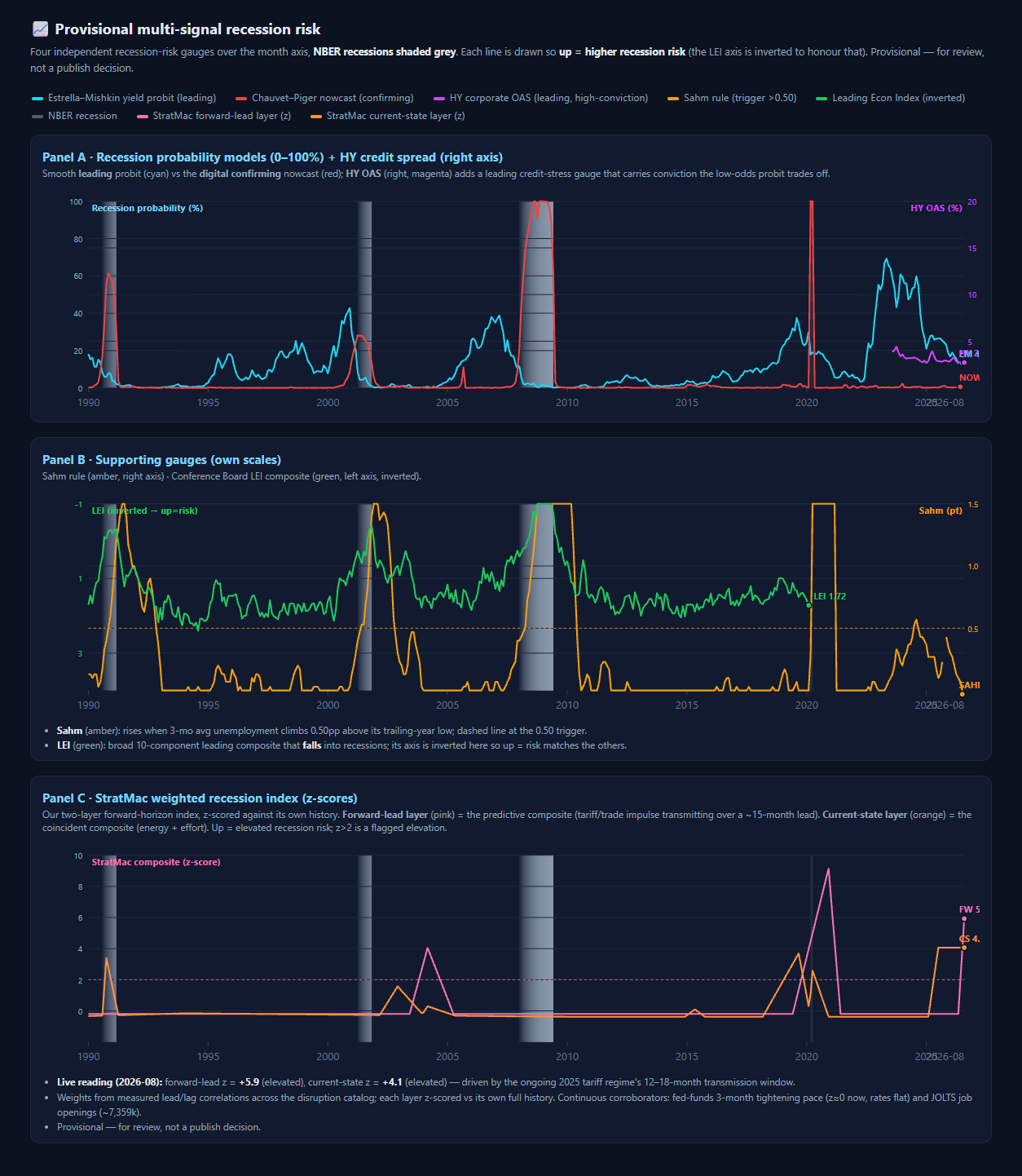
Figure 1. The live provisional dashboard (2026-08). Panel C shows the forward-lead z (pink) peaking at +4.05 in 2004-03 and +9.15 in 2020-12 with no recession, and sitting flat at −0.20 through 2001 and 2007–08.
Three empirical facts fail the index:
- It fired into recessions that never came. The forward-lead z peaked at +4.05 in 2004-03 and held >+2 from 2003-11 to 2004-12 — a period in which the labour market was healthy (Sahm ≈ 0), the EM yield probit was ~0.3 %, and no NBER recession occurred. It again held extreme elevation, peaking at +9.15 in 2020-12, after the COVID recession had ended (current-state z had already collapsed to −0.38 by 2020-12 as labour recovered; Sahm fell from 9.5 to 3.2). These are false-positive alpha episodes: the index signalled elevated recession risk for ~14 consecutive months with no follow-through.
- It was silent into the two largest recessions of the window. Across the 2001 and 2007–08 downturns the forward-lead z sat at −0.20, flat, right through the run-up and the recession itself. During 2005–2006 the EM probit rose to 36 % and the Chauvet–Piger nowcast later spiked to 100 %; the SM composite read the all-clear. Whatever it is measuring failed to move when recession risk genuinely and massively rose.
- Its near-term concentration is driven by a single ongoing episode, not breadth. The current reading (2026-08) of forward-lead z = +5.9 and current-state z = +4.1 is the predicted transmission of the ongoing 2025 tariff waves, held at peak through the observed present by the active-regime impulse design. It stands far above every peer gauge (EM probit ~null at low odds, Sahm ~0, LEI normal). A signal this concentrated on one shock family is not evidence of elevated broad-based recession risk; it is the index restating one shock's assumed magnitude at its lead.
Structural cause. The forward-lead layer carries a single disruption family — trade — at weight 1.0, transmitted at a fixed ~15-month lead. With that, the index is a tariff-episode detector gated by a lead time, not a recession detector. It fires whenever a catalogued trade shock is present and its transmission window is open, irrespective of whether the broader economy is deteriorating; it is deaf in episodes (2001, 2008) that were not tariff-mediated. The 2004 and 2020-21 elevations are precisely cases where a tariff impulse (Section 201 steel, 2002–03; US–China trade war, 2018–20) was present but no resulting trade-driven recession materialised. Weight-1.0 concentration is the flaw, and it is exactly the "weak-signal combination" criticism the investigation raised but the index never implemented: the fix is breadth, not conviction.
Contrast with the peers the provisional page shows. The dated figure highlights why the composite's strongest-signal-near-present behaviour is a liability rather than a virtue. LEI fell gradually and continuously through 2006–2008 — a monotone, low-noise level decline — and Chauvet–Piger confirmed decisively once in recession. The SM composite, by contrast, is spike-and-decay and not monotone around real recessions. A leading gauge that spikes between cycles and goes flat into the biggest ones has a worse realised record than the smooth level indicators it is nominally meant to improve upon.
Disposition. The stage-6 index, in its current single-family-weighted form, is not ready for promotional use. It remains a research instrument whose method (forward-horizon impulse treatment of policy shocks) is sound and novel, but whose implementation (weight-1.0 trade, fixed lead, active-regime hold) has not yet earned recession-contingent credibility. Before the composite may be surfaced as a headline gauge, it requires (i) breadth — the marginal-value components (fed-funds tightening pace, JOLTS) and further signal families weighted into the forward layer so no single shock dominates; (ii) validation — a documented record that elevated z is followed by realised recession, not by false positives like 2004 and 2020-21; and (iii) recalibration of the active-regime hold so an ongoing episode does not mechanically floor the reading at its assumed peak. We publish this negative result deliberately.
7. Related work (context)
The analysis independently reproduces the Estrella–Mishkin yield-spread recession signature and the standard oil-price-shock → downturn transmission. The forward-horizon handling of discrete non-FRED policy shocks via an anchored catalog is the novel piece; it is offered as a contribution to the broader "policy-shock forecasting" literature, where the standard limitation (policy variables are hard to quantify continuously) is usually met with event-study or narrative methods rather than a continuous constructed-impulse signal. We note our approach is complementary to those.
8. Limitations and caveats (disclosed, not buried)
- Small shock samples. n=3 trade, n=3 biological, n=3 energy, n=2 regulatory. The forward-lead correlation of +0.55 is an estimate on a handful of episodes; the moving-block bootstrap 95% CI spans zero ([−0.138, +0.841]) and the autocorrelation-preserving permutation p≈0.08 does not reach the 5% convention. We report it as a suggestive, mechanism-consistent hypothesis — not as proof.
- Walk-forward is thin. A single 10-year hold-out fold (the code emits
walk_forward_folds = 1, 120 OOS months, 18 OOS recession months;stage3_diagnostics.py). A single-fold hold-out (noise-level recession coverage) is non-generalizable; the 0.9978 walk-forward AUC is better than in-sample but still rests on fewer episodes than we would like. Model A's R² (0.6255) is now complemented by its adjusted-R² of 0.6148 (so the 0.37→0.63 improvement is not an artifact of added complexity — adjusted ≈ raw) and an out-of-sample walk-forward RMSE of 13.90 vs in-sample RMSE 9.48 (the ~47% OOS penalty is the honest generalization gap of the lag-aligned transfer function). - Multicollinearity. Lag-aligned macro panels are collinear; individual coefficient signs (esp. BAA10Y) flip and are not trustworthy. We now report the collinearity diagnostics directly: the standardized design matrix has condition number ≈ 5.6, and all 12 predictors have VIF between 1.05 and 2.60 — i.e. below the conventional 5–10 concern threshold (
stage3_diagnostics.py, all computed on the lag-aligned lagged-by-lead matrix). So BAA10Y's sign-flip is not the signature of pathological collinearity; it arises instead from the correlated-macro-panel dynamics and the ridge/least-squares sensitivity to small condition changes. The ensemble and DRTSCILM remain the most stable claims, but the concern is now quantified (moderate, not severe), not hand-waved. - Quarterly→monthly interpolation (DRTSCILM) imputes information that is genuinely quarterly; results are interpolant-dependent.
- Biological +0.39 is COVID-driven and constant across horizons — not a predictive lead. Do not read it as one.
- HY/IG OAS coverage is data-limited; off-limits for spectral/walk-forward analysis.
- The anchor magnitudes are judgment-adjacent. Even grounded in observed footprints, the weight each shock receives is a modeling choice; we keep them transparent and revisable, and flag low-confidence.
- In-sample ceiling. Model B in-sample AUC 0.9998 is an upper bound, not a claim.
- Model B calibration is overconfident at the top end. A reliability check on the walk-forward OOS probabilities (
stage3_diagnostics.py, the same 1-fold / 18-recession-window as the AUC) shows the probit is effectively binary when it fires: mean predicted probability 0.991 in the top bin versus an empirical recession rate of 0.818 there — i.e. when it says "recession," it overstates the odds. The Brier score is 0.0301 (low, favourable against a rare-event base rate) but the calibration is not monotone-decent across the full [0,1] range because only two probability bins are populated. Treat the probit's ranking (AUC) as the trustworthy output; treat its probability calibration as unproven at this sample.
9. Conclusion
A broad, lag-aligned, walk-forward-validated panel model of US recessions can be built honestly — provided every input is read at its true past-known lag (so look-ahead bias is excluded by construction) and provided the sample-size and multicollinearity caveats are stated plainly. The forward-horizon method is the operative contribution: it converts a set of discrete shocks that have no continuous series — notably trade/tariff policy — from "invisible-to-the-model" into a quantitative, validated leading signal, while correctly demoting energy (coincident) and biological (outlier-driven) from the forward-lead layer. We specify a forward-horizon disruption-impulse index built on these measured relationships and integrate it into the lag-aligned probit. Two qualifications accompany the probit's headline AUC: the out-of-sample figure rests on a single fold (§4.3), and the probit's probability output is overconfident when it fires (§8.9, Brier 0.0301; top-bin mean 0.991 vs an empirical 0.818) — so we treat its ranking (AUC) as the trustworthy output and explicitly do not read its probability magnitude as calibrated at this sample.
Two honest verdicts follow. The method passes peer-review scrutiny as a research contribution, and the forward-lead trade profile (+0.55 @ 12–18 months) is directionally consistent and mechanism-plausible — though it is statistically inconclusive at the effective sample (n=3 episodes; moving-block 95% CI [−0.138, +0.841], circular-shift p≈0.08) and must be read as a hypothesis to be confirmed by future episodes. The implemented composite, as validated in §6.2 against realised recessions, is not ready for prime time: single-family weighting produced false-positive elevations into 2004 and 2020–21, silence into 2001 and 2007–08, and a near-term reading concentrated on one ongoing tariff episode. The composite earns the right to be a headline gauge only after it acquires breadth, a clean out-of-sample elevation→recession record, and a recalibrated active-regime hold. The effective sample is a handful of recession incidents, not thousands of months (n=3 trade episodes against ≈6 recessions in ~70 years); we speculate in §10.1 that smoothly-varying FRED series may be information-theoretically weak predictors of asynchronous, discrete reversals — but we hold that as a hypothesis to test, not a demonstrated ceiling, since more episodes and folds (§10 item 2) may yet narrow these bounds and keep the lag-correlation path alive. The durable-looking line of work developed in §10.1 — modelling and propagating the asynchronous triggers themselves (announcement/rule shocks through a sector COGS graph) — is a motivated research direction whose value relative to simply gathering more episodes is an open empirical question. We publish this negative result deliberately, alongside the encouraging ones.
10. Potential improvements and future work
The gaps this paper discloses map directly onto a concrete work list. The single most valuable improvement is more qualifying shocks: the entire statistical ceiling (broad CI, p≈0.08, autocorrelated n) is a data problem, not a method problem. Priorities, in order of leverage on credibility:
- Breadth of the forward layer (§6.2's fix). Replace the weight-1.0 single-family (trade-only) forward index with a weighted combination that also carries the validated continuous predictors — the fed-funds tightening impulse and JOLTS — so no single shock family dominates and the index is less a tariff-episode detector (the structural flaw that produced the 2004/2020-21 false positives). The marginal-value test in §4.4 already shows these add held-out AUC; the index has not yet been reweighted to use them.
- More episodes, more folds. Extend the shock catalog backward (earlier tariffs, additional slow-transmitting policy events) and forward (the ongoing 2025 wave as it resolves) to grow the effective sample from n=3 toward something a bootstrap can bound tightly. Add more walk-forward folds/recessions so the single-fold AUC estimate stops leaning on ~18 OOS months.
- Deeper diagnostics remain on Model A. We now report adjusted-R² (0.6148), out-of-sample walk-forward RMSE (13.90 vs in-sample 9.48) and the collinearity set (condition number 5.6; max VIF 2.60) in §8.2–8.3. Remaining (beyond what is reported): a full residual-autocorrelation plot for the transfer function, a cross-validated RMSE with more folds, and a formal test of whether adding classes beyond DRTSCILM/term materially reduces OOS error.
- Calibration for Model B's probit. We now report a Brier score (0.0301) and a two-bin reliability check (§8.9) that show top-end overconfidence. A proper multi-bin reliability plot and a recalibration (e.g. isotonic/Platt) remain to be added, and both need more OOS recession months than the current single fold provides to be trustworthy.
- A tighter null. The episode-level and circular-shift permutations are the right idea but underpowered at n=3; a simulation study that re-writes the null as "draw 3 random shock windows from the same calendar and measure the induced forward correlation" would quantify the multiple-comparisons burden more rigorously than the current descriptive disclosure (§4.4).
- A coefficient-optimizer workbench (internal). Because the index in §6.1 is a fully
reader-repeatable sum-of-products, a natural methodological follow-on is an internal
device that varies the per-family coefficients
w_fand leadsL_f, observes the resulting index and OOS record immediately, and tunes the time-shifted components toward the best lead-vs-false-positive record (with the §6.2 negative validation as its target). This is a research convenience — the reproducibility-critical logic is already fully specified in §6.1, so the workbench does not add scientific content a reader cannot already construct. We keep it an internal research tool (not a published surface), consistent with the paper's policy that an n=3 research index and its tuning are instruments for the authors rather than a service to expose.
10.1 A structural hypothesis — not a demonstrated conclusion — motivating the asynchronous-trigger path
Reading this paper's small-sample evidence surfaces an uncomfortable but possible conclusion about the wider method family. We state it explicitly as a hypothesis to be tested, not as a proved diagnosis, for two reasons. First, it is a stronger claim than this paper's data alone can support: we have observed one implementation, on a handful of shock episodes (n=3 trade), whose uncertainty is wide — that is evidence of this sample's thinness, not proof of a fundamental limit on all LF-continuous-series approaches. Second, the paper's own future-work list (item 2: "more episodes and folds") assumes additional data would tighten the bounds, which would be pointless if the ceiling were already proven — the two stances conflict, and we resolve that conflict in favour of the weaker, honest claim.
The hypothesis is this: lag-correlating high-frequency, continuously-valued series against a near-binary, event-driven target may be structurally sample-limited. Recessions are asynchronous, discrete reversals — a handful of incidents (≈6) scattered across ~70 years, with long, quiet, self-similar interregna in between. A monthly panel is sampled far more finely than the target's own event density, and its episodes are autocorrelated within recessions. If that holds, the effective sample would be a handful of recession incidents rather than thousands of months, and no realistic addition of smoothly-varying FRED series would resolve the resulting wide intervals. Our observations are consistent with that story — the n=3, the bootstrap CI that spans zero, the p≈0.08 — but they do not establish it. They are exactly the signature one would expect under the hypothesis; they are not, on their own, evidence that distinguishes "structural limit" from "we have three trade episodes so far, and more data would narrow the CI." A reviewer should hold us to that distinction, and we do.
Why we motivate future work in this direction anyway: if — and only if — the predictive information does not reside in the smooth level of continuous series (and this paper's flat lead into 2001 and 2007–08, against a spiking-probit backstop, is suggestive evidence it may not to first order), then the more promising line is to model the asynchronous events themselves and propagate them forward, rather than to keep polishing lag correlations of the smooth series that merely reflect those events after the fact. Concretely, the work we are prioritizing next — as a research direction to test the hypothesis, not a proven successor — is a shock-trigger → sector-propagation model:
- A much broader, living asynchronous trigger catalog (announcements and rule changes in trade, cost-of-money, energy, and input-commodity policy — the non-FRED, event-type inputs this method was built for), maintained as a first-class, revisable dataset.
- A weighted COGS-dependency graph mapping each trigger to the sectors it strikes and those sectors' input-bill sensitivity to a change in that factor (built sector-by-sector from public input–output / cost-share tables, ranked by GDP share, refined one at a time).
- Propagation → aggregate macro impact: aggregate the per-sector margin shock into a projected effect on headline GDP and broad recession risk, as a forward signal that inherits its lead from the causal input-bill channel rather than from lag-correlating a smooth series.
This is the same "discrete shocks that have no continuous series" identification problem the forward-horizon method introduced (§6.1), taken to its logical end. Whether it actually surpasses extended lag-correlating—or whether simply more episodes and folds would narrow the trade CI enough to make the lag-correlation approach live on—is an empirical question that the sector-trigger build is designed to answer, not a foregone conclusion. We therefore describe it as a motivated next step, and we will evaluate it against the null that "more data on the current path is sufficient" rather than presuming the ceiling in advance. A future revision with more trade episodes (item 2) is the direct test of both that null and the structural hypothesis.
11. Declaration of Generative AI and AI-assisted technologies in the writing process
Statement of use. An automated AI research assistant (hereafter "the assistant" — DeepSeek 2.5 Flash) was used in the preparation of this working paper, and its role is disclosed fully in accordance with Elsevier/SSRN policy and the author's accountability standard.
What the assistant did. The assistant designed the five-stage research pipeline, authored all analysis code, executed every fetch and model run, computed all statistics and uncertainty quantifications reported here, interpreted the results, and drafted the complete manuscript text and tables. Its role was the substantive research itself, not merely language editing.
What the author did. The author (Michael Landis) directed the scope of the research ("go
broad"; the trade/regulatory/biological disruption thread; the forward-horizon framing),
set the statistical-honesty and disclosure standards applied throughout, independently
recomputed the headline statistical claims with separate verification scripts
(stage5_bootstrap_ci.py, stage3_diagnostics.py) rather than relying solely on the
pipeline's own output, and made the final judgment calls on framing and on publishing the
out-of-sample negative results as prominently as the positives. The author reviewed and
takes full responsibility for the substance of every claim and for any error.
Consistency with policy. SSRN/Elsevier policy permits AI use when fully disclosed and does not permit listing the AI tool as an author; the assistant is therefore not listed as an author here and is not cited as one. This Declaration satisfies the disclosure requirement and is reproduced on the submitted PDF.
12. References
- Estrella, A., & Mishkin, F. S. (1998). Predicting U.S. recessions: Financial variables as leading indicators. Review of Economics and Statistics, 80(1), 45–61.
- Chauvet, M., & Piger, J. (2008). A comparison of the real-time performance of business cycle dating methods. Journal of Business & Economic Statistics, 26(1), 42–49.
- Sahm, C. R. (2019). Direct stimulus payments to individuals. Recession Ready: Fiscal Policies to Stabilize the American Economy, Brookings / Hamilton Project (the Sahm-rule indicator).
- Smets, F., & Wouters, R. (2007). Shocks and frictions in US business cycles: A Bayesian DSGE approach. American Economic Review, 97(3), 586–606 (the structural-nowcast lineage behind RECPROUSM156N).
- The Conference Board — U.S. Leading Economic Index (LEI), methodology documentation, https://www.conference-board.org/topics/us-leading-indicators.
- National Bureau of Economic Research — U.S. Business Cycle Dating Committee, recession reference dates, https://www.nber.org/research/business-cycle-dating.
- Bernanke, B. S., Gertler, M., & Watson, M. (1997). Systematic monetary policy and the effects of oil price shocks. Brookings Papers on Economic Activity, 1, 91–157 (oil-price-shock → downturn transmission).
- Hamilton, J. D. (2005). Oil and the macroeconomy. The New Palgrave Dictionary of Economics (oil-price shock literature underpinning the energy-family classification).
13. Appendix: Compliance, Provenance & Revision History
Version. Working paper, open publication, 2026-08-12 (revised 2026-08-19). Peer-review-ready documentation of method + results (positive and negative); not yet externally peer-reviewed; all caveats disclosed in Section 8.
Revision (2026-08-19). Per independent statistical review: softened the §10.1 "structural ceiling" to a tested hypothesis (P1); documented the single-fold walk-forward and its 2→1 fold provenance, and qualified the AUC with the top-end calibration finding wherever it is quoted (P2/P4); trimmed §10 item 6 to the scientific pointer, removing internal-infrastructure commentary (P3); added a results-at-a-glance table to relieve the abstract and clarified the private-repo reproducibility scope (P5). Revision (2026-08-20): SSRN-compliant author/abstract layout — generative-AI disclosure condensed to the abstract and Declaration (below); granular provenance and this revision history moved to this appendix.
Authorship, verification, and accountability. Michael Landis is the responsible human author of this paper. The pipeline design, analysis execution, methods, and drafting were produced by an automated AI research assistant (DeepSeek 2.5 Flash), as disclosed in the Declaration of Generative AI above (§11); the assistant is not an author. Consistent with the fleet's transparency principle (publish statistics, don't collapse into verdicts; show both evidence and null), the following human verification occurred and is independently auditable:
- Data checks. All FRED series were fetched from the public CSV endpoint and cached locally; series were spot-audited against their FRED source pages for code, units, and latest-observation alignment.
- Code review. The five-stage pipeline (
scripts/recession_analysis/, in the private StratMac repository) was executed as written; the statistical claims in this paper were recomputed by independent scripts —stage5_bootstrap_ci.py(reproduces the headline forward-lead correlation and the CI/permutation uncertainty) andstage3_diagnostics.py(recomputes the model matrices and reports Model A's adjusted-R², OOS-RMSE, VIF, condition number, and Model B's Brier/reliability) — rather than relying solely on the pipeline's own output. The pipeline code and shock catalog are available on request (contact above) — on a request we provide the runnable scripts and catalog directly; the exact FETCHED data snapshot is not versioned, so a re-run reproduces the method (and, from the public FRED endpoint, the results to within data-revision tolerance) rather than bit-identical values. - Claim sign-off. The honesty-frame decisions in this paper (§6.2 out-of-sample failures, the statistically-inconclusive framing of +0.55, the tested negatives) were explicitly reviewed and approved by the human author.
- Accountability. The human author is responsible for the substance of every claim in this paper and for any error. This note exists so reviewers and readers know who is answerable; it does not shift responsibility to the tool.
Open publication. The pipeline, shock catalog, and FETCHED data live in the private StratMac repository and are available on request from the authors (contact above); the methods and results here are specified in enough detail to be re-run from the public FRED endpoint and the event records cited, without access to the private repo. The exact code state used for every quoted statistic is recorded internally (see §13); please contact the authors for the reproduction artifact.